In a sense, computational materials science performs virtual “measurements” of a material given a description of its structure. While many such computational measurement techniques have been developed, density functional theory (DFT) is now the most popular approach to rapidly screen compounds for technology. DFT solves quantum mechanics equations that determine the behavior of electrons in a material (approximately); these electron interactions ultimately determine the material’s chemical properties. Compared to other theories, DFT strikes a good balance in terms of being accurate, transferable (not needing too many tweaks for different materials), and low in computational cost^[1].

Yet, it is all too easy to list shortcomings of density functional theory. One can only model a repeating unit cell containing about 200 atoms; beyond this, the computational cost of using DFT very rapidly becomes unattainable. Thus, with DFT the richness of materials behavior at larger length scales is lost. Even for materials that can be described with so few atoms, DFT calculations are often subject to large inaccuracies. Unfortunately, there is no theory to tell you how accurate or inaccurate a particular DFT calculation will be. Finally, with computational screening you are usually unsure if the materials you designed in a computer can ever be synthesized in the lab.

With all these limitations, how should a materials researcher interpret DFT results?

Materials cartography

One might view the results of density functional theory predictions in the same way he or she might set sail with an old map of the world. That is, as a useful guide that should be taken with a healthy grain of salt. For example, we can draw parallels between Ptolemy’s 2nd century world map and the current state of the art in high-throughput calculations.

Certain regions of the world are mapped better than others. Ptolemy’s map gets the northern Mediterranean roughly correct, but then starts failing catastrophically in the southern region. The Black Sea is quite accurate; the Caspian Sea is entirely wrong. Similarly, DFT works quite well for metals and many semiconductors and insulators, but starts to become very unreliable for strongly correlated materials (such as superconductors). How much you trust DFT really depends on what region of the “materials world” you are in.

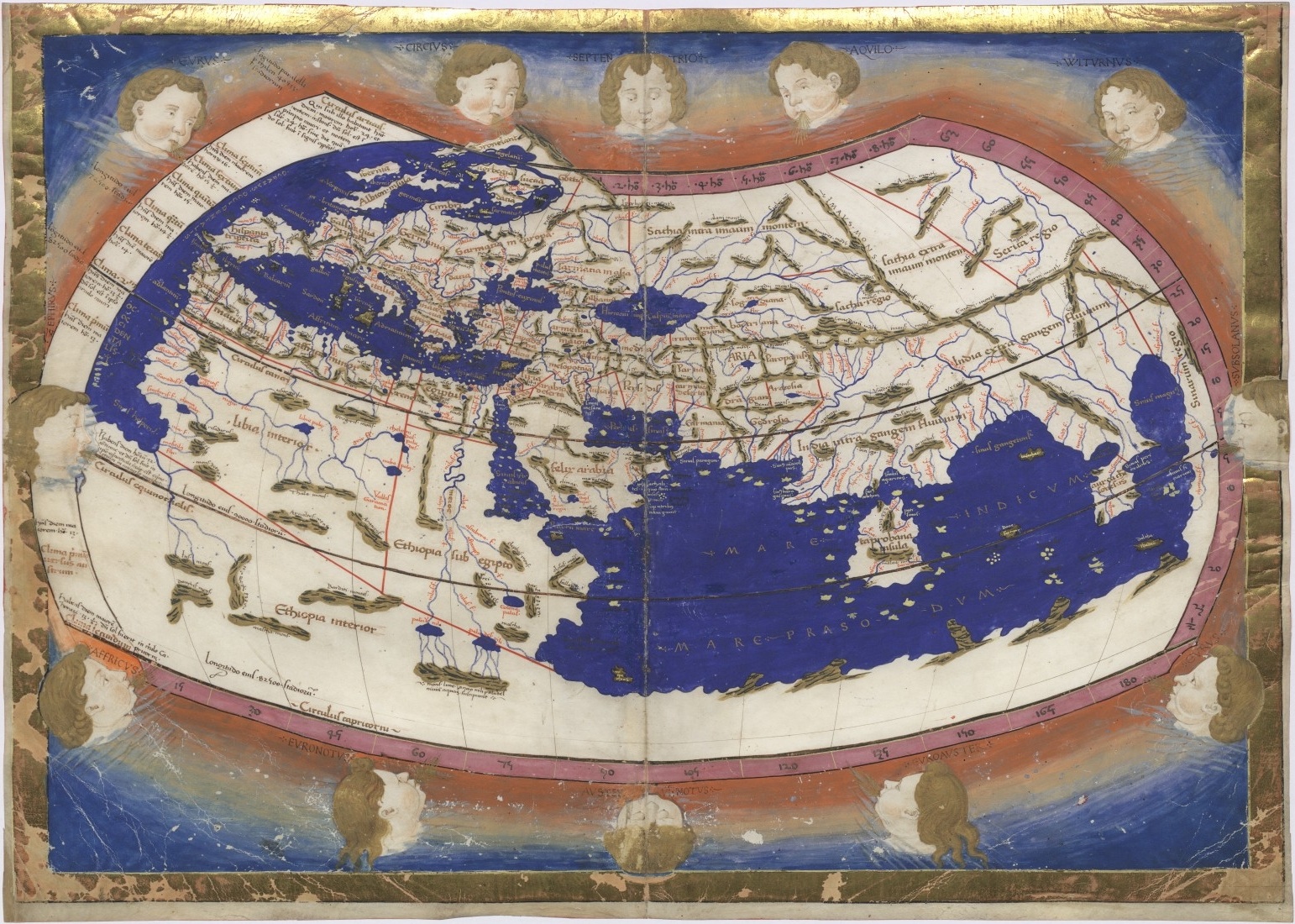
Sometimes, the overall trend is correct, but the fine details are lacking. The shape of the Arabian Peninsula in Ptolemy’s map is approximately correct but doesn’t get the details right. This is often the case for certain properties computed by density functional theory. For example, when optimizing the coordinates of the atoms in a material’s structure, DFT often slightly under-predicts or over-predicts the bond lengths, but usually gets the overall solution remarkably close to that seen in experiments.

Other times, the trend can’t be trusted, but some fine details can still be recovered. The width of the Red Sea on Ptolemy’s map is not represented faithfully, particularly how it widens severely at the bottom. Yet, certain details like the Gulf of Aden can be seen from the map, and the coastline (particularly the eastern one) is not too bad. Similarly, with some materials properties (such as the band structure), DFT often misses the big picture (width of the  energy gap between conduction and valence bands) but recovers some useful details (e.g. general shape of the bands on either side, and their overall curvature).

Entire swaths of the world are completely missing. Just as the sailors of Ptolemy’s day had not ventured out to all parts of the world yet, DFT computations have not yet been performed across all potential materials. With high-throughput DFT, we are essentially sending hundreds of ships in every direction to look for entire new materials continents filled with hidden riches. However, we can’t say that the map is complete.^[2]

If you are an experimentalist and are going to set sail with a DFT-based map, you’d better have a sense of adventure and realize you might have to correct course based on what you see. You might also want to get some previous guidance about the sketchier areas of the materials world. But, you’d probably rather have the map than rely only on your personal knowledge of the seas.

Slaying the dragons and sea monsters

In earlier days of mapmaking, it was not uncommon to place drawings of monsters over uncharted regions, warning the seafarer to proceed at their own risk (hence the popular phrase, “Here be Dragons”^[3]). A similar warning might apply today to experimentalists interpreting DFT maps for excited state properties and strongly correlated materials.

Yet, the DFT version of the materials world is growing closer to the truth with time. While certain “monsters” remain unslayed for decades, brave DFT theorists have wounded many of them (and been knighted with a PhD). Over time, as DFT techniques improve, the monsters will start to disappear from DFT maps^[4]. And as high-throughput computations set sail for new materials in new directions, more classes of interesting technological materials will become known to us. Our maps are not perfect, but they will continue to improve; in the meantime, experimentalists will have to retain their sense of adventure!

Footnotes:
[1] The amount of time needed to compute the properties of a single material depends on the material’s complexity and on the number and type of properties desired. A reasonable range is between 100 CPU-hours (1 day on your laptop) and 10,000 CPU-hours (100 days on your laptop).
[2] For more details on why we can’t compute everything, see the previous post on “The Scale of Materials Design”.
[3] Despite being a great phrase, “Here be dragons” apparently wasn’t used that much on old maps.
[4] For an example of how DFT is progressing into difficult territory, see this recent prediction of a new superconductor.